The Idea That Was Supposed to Fail
Why DirectFlash and Evergreen//One suddenly look a lot smarter in a world of NAND and DRAM price shocks Dmitry Gorbatov Mar 20, 2026 Important Note for my readers: Writing this piece took me a lot longer than I normally spend on a post. It took a lot of reading and research. Many articles and blogs were written on the subject before NAND and DRAM costs went crazy. The dry-humor version is that the storage industry spent years insisting flash was just disk with better manners, and then acted surprised when the underlying physics eventually asked to speak with management. Now, let’s get to it. I can still picture the room. It wasn’t anything special — just another corporate competitive training session, the kind you’ve sat through many times if you’ve spent enough years in enterprise tech. This was at NetApp, in 2015 or 2016, back when flash was still a question mark. Not if, but how. The industry had not fully committed yet, and everyone was trying to figure out what role it would play. The presenter clicked to the next slide, paused for a second, and said something that stuck with me in a way most of those sessions never do: “Pure Storage is crazy! They’re building their own flash modules. That’s stupid. It’s not sustainable. They won’t survive.” It wasn’t said for effect. There was no dramatic pause afterward, no attempt to persuade. It was delivered as a simple, almost obvious conclusion. And to be fair, it felt obvious. Because the entire storage industry operated on a shared assumption: you didn’t build components, you assembled them. You relied on a mature ecosystem of suppliers who specialized in drives, storage controllers, and memory, and you focused your differentiation on software features and integration. That was the efficient path. That was the scalable path. That was how serious companies behaved. What Pure was proposing at the time — what would later become Everpure — felt like a deviation from that logic. Building your own flash modules didn’t just introduce complexity; it seemed to reject the economic advantages of the broader supply chain. It looked like a risk without a clear payoff. So the conclusion made sense. Until it didn’t. Looking Back, Differently If I think back to that training session now, I do not really see it as a moment where someone was foolish. I see it as a moment where the industry was trapped inside the logic of its own assumptions. If you believe flash should look like disk, then building your own flash modules sounds silly. If you believe storage is just a sequence of refresh cycles, then a model built around non-disruptive evolution sounds unnecessary. If you believe component pricing will keep trending in the right direction forever, then architectural efficiency feels like an academic luxury. But once those assumptions start to crack, the logic changes. And when it changes, the things that once looked eccentric start to look oddly prescient. A Change You Don’t Notice Right Away For years, nothing about that statement felt particularly worth revisiting. The industry moved forward in predictable ways. Flash became mainstream. Performance improved. Density increased. Vendors competed on features, benchmarks, and price points. The conversations most of us had with customers followed familiar patterns. If anything, the abstraction layers built around flash made things easier to consume. SSDs behaved like faster disks — and that was good enough. There is a reason they showed up in familiar HDD form factors. The industry was trying to preserve the old world while sneaking in a new medium. Keep the slots. Keep the enclosures. Keep the assumptions. Change as little as possible. That made adoption easier, but it also buried the problem. Because flash is not a disk. It never was. It does not behave like one, and it does not particularly enjoy being treated like one. The only reason the illusion worked is because the industry built a fairly elaborate translation layer to maintain it. That translation layer is where the story really starts. The Trick That Made Flash Look Simple When commodity SSDs became the standard way to bring flash into enterprise storage, they depended on a piece of internal firmware called the Flash Translation Layer, or FTL. Its job was deceptively simple: make raw NAND look like a disk. That sounds harmless enough until you think about what that actually requires. NAND cannot just overwrite data in place the way the rest of the stack would like it to. It has to handle erase cycles, wear leveling, garbage collection, bad block management, and the constant translation between logical addresses and physical locations on the media. So every SSD became its own little self-contained world, complete with its own controller, its own metadata tables, and its own DRAM to keep track of everything. In other words, every drive became a tiny independent computer, making local decisions in isolation. That design solved the adoption problem. It did not solve the architecture problem. For a while, the tradeoff seemed worth it. The drives were fast enough, the packaging was familiar, and the whole system kept pretending that flash was just a much nicer version of disk. But what looked neat and modular at small scale turned out to be awkward and expensive at enterprise scale. And that is where the “stupid” decision begins to look a lot smarter. What Commodity SSDs Actually Drag Along With Them The more I researched this topic (and believe me I did), the more I realized how much of the industry got comfortable with an abstraction that was doing a lot of quiet damage. Commodity SSDs carry four structural inefficiencies that matter much more today than they did when pricing was stable. Trapped DRAM. Every SSD maintains its own mapping tables, so large-scale systems end up carrying a remarkable amount of DRAM inside the drives themselves. That memory is necessary for the SSD to function, but it does not really help the array think globally. It is duplicated overhead, repeated again and again, drive by drive. In a petabyte-scale system, that is not a rounding error. It is cost, power, and complexity hiding in plain sight. Unpredictable Latency. Garbage collection inside a traditional SSD happens when the drive decides it needs to happen. When that occurs, the drive may become temporarily less responsive, and in an array full of independent drives, those little stalls start to show up as tail-latency spikes. The system is always vulnerable to one drive having a private crisis at exactly the wrong time. Write Amplification. Because the SSD does not really understand the workload or the data structures above it, it moves data more often than necessary. More movement means more writes. More writes mean more wear. More wear means the media gets consumed faster than it should. Over-provisioning. Every SSD holds back some raw capacity for its own housekeeping and spare-cell management, but that reserved space is siloed. The array cannot use it intelligently across the system because each drive is managing its own private affairs. None of this sounded especially dramatic when NAND kept getting cheaper and the economics of flash kept improving. It sounded like engineering trivia. The sort of thing infrastructure people argue about while everyone else waits for the quote. Today it is not trivia. Today it is exposure. Why AI Made This Suddenly Everyone’s Problem For years, one of the quiet assumptions in enterprise IT was that storage capacity would continue to become cheaper and more abundant over time. Not perfectly, not smoothly, but predictably enough that the inefficiencies of the underlying architecture could be tolerated. That assumption is now not only under pressure, it is getting decimated. AI did not just create a new category of interesting workloads. It created a global appetite for silicon that is large enough to bend supply curves. The cute part of AI is easy to mock. The cat kicking the T-Rex. The surreal generated videos. The deepfakes that make you look twice and then sigh a little for civilization. But behind every one of those outputs is a less funny reality: extraordinary consumption of DRAM, NAND, GPUs, and supporting infrastructure. The novelty at the edge is powered by very serious resource demand at the core. And that demand is landing directly on the components enterprise storage depends on. This is the part customers are beginning to feel in ways that are no longer abstract. Expansion quotes do not look as comfortable as they once did. Refresh cycles feel more expensive. Delivery windows stretch. Budgets built on assumptions from even two years ago suddenly need more explaining than anyone wanted. There is a tendency to call this inflation because that is the easiest word available. It is not really inflation. It is supply and demand, with a side of semiconductor reality. And that matters, because a traditional SSD array is exposed to both sides of the problem at once. It is exposed to NAND because that is the medium you are buying, and it is exposed to DRAM because every SSD drags its own DRAM overhead along for the ride. When those two markets tighten at the same time, the cost of the architecture gets hit twice. That is not just a technical nuance. That is economics. Revisiting the “Stupid” Decision This is where the old training-room comment starts to age badly. Because what looked like unnecessary vertical integration was really a decision to stop pretending flash was a disk and start treating it like what it actually is: semiconductor media with very specific physical behaviors that should be managed at the system level, not hidden inside dozens of drives. That is the DirectFlash idea in plain English. Take the Flash Translation Layer out of the individual drive. Pull media management into the operating environment. Let Purity manage flash globally instead of leaving each device to improvise its own local strategy. That changes more than performance charts. It means metadata no longer has to be duplicated and trapped inside every SSD. It means wear leveling can happen across the full system instead of inside the borders of a single device. It means bad block handling, garbage collection, and data placement can be coordinated with global context. It means the platform can see the difference between data that should live together and data that should not, which dramatically reduces unnecessary movement and lowers write amplification. And when write amplification drops, the economics change. The NAND lasts longer. The useful life of the media extends. Lower-endurance flash, like QLC, becomes viable for serious enterprise use because the software is smart enough not to abuse it. The system extracts more useful work from the same raw silicon. That is not just clever engineering. That is insulation from volatility. The reason this matters now is that DirectFlash changes the ratio between the silicon you buy and the value you get from it. If the rest of the market is paying more for NAND and more for DRAM, an architecture that reduces trapped DRAM, minimizes wasted writes, extends media life, and packs far more capacity into far denser modules is not just elegant. It is economically defensive. This is where the old “they build their own flash” criticism misses the point. Building your own flash modules was never the point by itself. The point was controlling the relationship between software and media well enough to eliminate the inefficiencies the commodity model had normalized. Why Purity Is the Real Story DirectFlash makes for a good visual. It is a module. You can point to it. You can talk about density and reliability and the fact that a 150TB module can do work that would have required a small army of traditional devices not all that long ago. But the real story is Purity Operating Environment, i.e. software. Purity is where the architectural bet pays off. It is what turns raw NAND into a coordinated system instead of a pile of politely disagreeing SSDs. Because Purity sees the entire media pool, it can write more intelligently. It can group data with similar expected lifespans together, so that when a snapshot or a temporary workload disappears, whole regions of storage can be retired cleanly instead of forcing background reshuffling of still-live data. That reduces unnecessary churn. Less churn means fewer writes. Fewer writes mean longer media life. Because Purity sees when a NAND die is busy with an erase or program cycle, it can avoid letting that become a host-visible performance problem. RAID-3D and system-level awareness allow the platform to reconstruct data from parity rather than simply waiting for a busy drive to get its act together. The end result is deterministic performance rather than a roulette wheel of occasional latency spikes. Because Purity owns media management globally, the over-provisioning and spare resources are no longer trapped in per-drive silos. The system can use them strategically. I know that all of this sounds a bit scientific, and to be fair, it is. I did spend over 7 years working for Everpure and a few weeks researching for this post. I wanted to sit with that science for a bit. Where the Economics Start to Matter The moment component pricing becomes unpredictable, architecture stops being an engineering preference and starts becoming a financial strategy. That is the part that matters most to customers right now. A traditional buying model assumes that at some point you will hit a refresh cycle, a capacity wall, or a migration event that forces a purchase whether the market timing is good or terrible. You buy when you have to buy. If NAND is expensive, that is unfortunate. If DRAM is expensive too, even better, because apparently the universe enjoys symmetry. That is what makes the combination of DirectFlash and Evergreen so important. DirectFlash reduces the amount of waste, duplication, and premature wear in the system. Evergreen removes the old habit of tying innovation to forklift replacement. Controllers evolve. Capacity can be consolidated into denser modules over time. Data stays in place. The customer is not forced into rebuying the whole environment every few years just to remain current. That already changes the economics. But it still leaves one more question: who is carrying the price risk? And this is where Evergreen//One matters more than ever. The Part I Actually Wanted to Get To Evergreen//One is not just a consumption model. It is not just a nicer way to finance storage. It is a mechanism for moving volatility away from the customer. That is the conclusion I wanted to earn, not just declare. When NAND and DRAM prices start climbing, most traditional models push that turbulence straight into the customer’s planning cycle. The customer eats the increase, absorbs the uncertainty, and tries to explain to the business why the infrastructure line now behaves like it has a gambling problem. Evergreen//One changes that relationship. The customer consumes capacity as a service. Everpure owns the burden of the underlying hardware lifecycle, the media strategy, and the ongoing optimization. DirectFlash makes that model stronger because the platform is structurally more efficient with the silicon it uses. It needs less trapped DRAM, wastes fewer writes, extends media life, and supports denser modules that deliver more usable capacity per unit of power, space, and raw media. Purity compounds that advantage with data reduction, ongoing software improvements, and smarter system-wide media management. Put differently, Everpure is in a much better position to absorb and manage component volatility than a customer buying boxes on a refresh schedule. That is the real price protection story. Not some magical promise that economics no longer apply. They do. NAND still costs what NAND costs. DRAM still costs what DRAM costs. Physics remains annoyingly undefeated. The difference is who is exposed to that volatility, how much inefficiency is built into the system before the customer ever sees it, and whether the operating model gives the customer a stable runway instead of a quarterly surprise. DirectFlash reduces the waste. Evergreen removes the forced disruption. Evergreen//One shifts the risk. That combination is a lot more interesting than it sounded in that room 11 years ago. The Part I Didn’t Appreciate Then What I did not understand sitting in that room 11 years ago was that some decisions are made for futures that have not arrived yet. The market eventually caught up to the architecture. That does not happen often enough in enterprise tech to ignore when it does. DirectFlash was never interesting just because it was different. It was interesting because it removed layers of inherited inefficiency that the rest of the market had accepted as normal. And in a period where NAND and DRAM pricing are under pressure, removing inefficiency is no longer just a performance story. It is a protection story. That is why this matters now. Not because it makes for a clever slide. Because it gives customers a more predictable way forward when the underlying component markets are anything but predictable. And in the current environment, that might be the most practical definition of innovation there is. Appreciate you reading. Dmitry Gorbatov © 2025 Dmitry Gorbatov | #dmitrywashere649Views3likes1Comment
The Art of Sizing: How to Size an Exadata Migration Without Overbuying Storage
If you are moving Oracle databases off Exadata, the first sizing mistake is usually looking at only one database at a time. Exadata is not a traditional Oracle architecture. Some of the work that would normally happen on the database host is performed by the storage cells, including capabilities such as Storage Indexes, Smart Scan, and—depending on the database version and workload—vector offloading. That changes what the storage numbers mean. A successful migration therefore needs to answer two different questions: How much I/O is the current Exadata environment really performing? Which parts of that work will move to the database hosts, change shape, or disappear when the architecture changes? This installment of The Art of Sizing walks through a practical way to answer both questions. Why Exadata sizing is different In a conventional Oracle environment, it is common to begin with the database-level system statistics and identify the read and write workload for that database. That is still useful on Exadata, but it is not enough. Exadata is often a consolidated platform running multiple databases across multiple storage cells. The migration target must be sized for the estate as a whole, not just for whichever database happens to be easiest to measure. The other difference is architectural: Exadata reports include physical work performed by the cells. That work can include processing that a non-Exadata design may need to perform elsewhere. The implication is simple: Do not copy an Exadata number directly into a replacement-storage calculator and assume the result is equivalent. First, understand what the number includes. Then normalize it for the target architecture. Start with the familiar metrics—but use the global view For a normal Oracle workload, the starting point is the System Statistics (Global) view. The key measurements are: Read IOPS: physical read total IO requests Write IOPS: physical write total IO requests Read MB/s: physical read total bytes Write MB/s: physical write total bytes These measures establish the workload profile, but a per-database view can hide the scale of a consolidated Exadata environment. Figure 1: The Global Activity Statistics view provides the starting point for reading Oracle read and write activity. The detailed statistics show the specific physical-read and physical-byte measures that should be carried into the analysis. Figure 2: Example physical-read measures from the global statistics output. The important word here is global. If Exadata is hosting several databases, collect the workload across the full environment. A replacement platform must be able to absorb the combined demand, including concurrent peaks that may not be visible when databases are reviewed independently. Use the Exadata AWR Global RAC report to see the platform as a whole The Exadata AWR Global RAC report is valuable because it brings the consolidated environment into view. It shows the disk types, cell counts, disk counts, IOPS, and bandwidth associated with the Exadata storage layer. In the example from the source report, the cells are performing approximately: 615,244 IOPS 28,899 MB/s Those values come from the F/6.2T and H/20.0T disk groups shown in the report: 404,115 IOPS plus 211,129 IOPS equals approximately 615,244 IOPS 24,297 MB/s plus 4,602 MB/s equals approximately 28,899 MB/s Figure 3: Example Exadata storage-cell performance summary. These are useful sizing inputs, but they are not automatically the final requirements for the migration target. They describe the physical work being performed inside the Exadata architecture. That distinction matters because Exadata is doing more than simply storing blocks. Account for the work Exadata is doing for you When you leave Exadata, some of the platform behavior may need to be reproduced through database design, host resources, or application changes. The exact impact depends on the workload, database version, SQL mix, and target architecture, so the assessment must be validated with the DBA and application teams. Exadata capability or behavior Migration sizing question Storage Indexes Will equivalent filtering be provided by indexes, partitioning, clustering, or SQL changes? Smart Scan Will more data be returned to the host because the target platform does not perform the same cell-side filtering? Vector offloading Where will vector-related processing occur, and what CPU, memory, and I/O will it require? Consolidated storage cells Will the target platform handle the same concurrency and peak overlap across all databases? Large SGA requirements Does the target need additional host memory to preserve cache behavior and avoid turning cell-side efficiency losses into repeated reads? Table and index layout Do large tables need new indexes, partitioning, or access-path changes to deliver comparable performance? This is the part of the migration that is easiest to underestimate. The goal is not merely to reproduce the observed Exadata I/O. The goal is to understand the work behind that I/O and decide where it will run after the migration. Normalize ASM redundancy before sizing capacity The Exadata summary also shows how much storage is allocated and used through ASM. This is where capacity can be overstated if the redundancy model is carried into the new architecture without question. The source example uses ASM High Redundancy. In ASM, that means the database data is stored with three copies. If the target storage platform supplies its own protection and the design uses ASM External Redundancy, the database layer may need only one logical copy. Figure 4: Example ASM disk groups with High Redundancy and their allocated and used capacity. As a first-order capacity normalization, moving from three ASM copies to one logical copy reduces the ASM-replicated requirement by approximately 66.7 percent. For example, 600 TB represented under a three-copy ASM model could correspond to roughly 200 TB of logical database data before adding target-platform protection, snapshots, growth, recovery copies, and operational headroom. That is not a universal storage-sizing answer. It is a normalization step. Before using it in a purchase or design, confirm: Whether External Redundancy is appropriate for the target architecture How the storage platform protects data and handles failure domains Whether the design includes snapshots, replication, backup staging, or disaster recovery copies How much free space and growth headroom the environment requires Whether the capacity numbers are raw, usable, allocated, or actually consumed The key lesson is that database redundancy and storage redundancy should be evaluated together. Counting both without understanding the division of responsibility can lead to buying protection twice. Do not reduce performance by the same percentage automatically It is tempting to apply the same 66.7 percent reduction to IOPS and MB/s because the ASM model moves from three copies to one. That can be a useful initial hypothesis, but it is not a guaranteed performance result. Read and write behavior can change differently. Exadata cell processing may be removed. Host-side indexes or partitioning may add work. The target storage platform may also use a different protection scheme, data-reduction method, caching model, or concurrency profile. A better approach is to use the Exadata numbers as a measured baseline, then build a target model with explicit assumptions: Baseline physical read and write IOPS Baseline read and write bandwidth Peak and average behavior across the full database estate Expected change in host-side processing Expected impact of indexes, partitioning, and larger SGA requirements Target protection and redundancy model Growth, recovery, and availability requirements That model gives the migration team something it can test instead of a single inflated number or an overly optimistic discount. A practical Exadata migration sizing workflow The process can be summarized in six steps: Collect the Global RAC and Exadata AWR reports for the full environment. Record average and peak IOPS, bandwidth, storage utilization, disk types, and database concurrency. Separate database workload from Exadata cell-side processing and identify what may move to the hosts. Normalize ASM redundancy so database copies are not counted twice with storage protection. Add target-specific requirements for CPU, memory, indexes, partitioning, snapshots, replication, recovery, and growth. Validate the model with short-window performance data and a representative migration or proof of concept. The first four steps create the sizing baseline. The last two turn that baseline into a design that can survive real workloads. The sizing lesson Exadata migration sizing is not a matter of copying the largest number from an AWR report into a storage proposal. It is an exercise in separating three things: The work the current environment is performing The protection and redundancy that are being counted today The work and protection the target architecture will need tomorrow In the example discussed here, the Exadata cells show roughly 615,244 IOPS and 28,899 MB/s, while the ASM configuration indicates High Redundancy with three copies of the data. Those are important facts, but they are starting points—not automatic target requirements. The most reliable design is the one that measures the whole estate, understands the Exadata features behind the measurements, removes duplicated redundancy, and then adds back the host, protection, recovery, and growth requirements of the destination platform. That is the art of sizing an Exadata migration: not buying for the biggest number, but understanding what the number actually represents. Final thought When an Exadata migration is undersized, the problem usually appears after the architecture is already difficult to change. When it is oversized, the organization pays for capacity and performance that may never be used. The better path is disciplined normalization. Measure Exadata as a consolidated system. Identify which work will move. Separate database redundancy from storage protection. Then size the target for the workload you are actually building—not the architecture you are leaving behind. That is how sizing turns a migration estimate into an engineering decision.56Views0likes0CommentsAccelerate 2026 - Part 1 - Everyone Wants Your Data
Back in February, I wrote that I had never been to Pure//Accelerate. This year, I still am not in Las Vegas. I watched the Everpure Accelerate 2026 opening keynote live from my home office, which turned out to be a different kind of vantage point. Not better than being there. Not worse. Just different. You do not get the hallway energy. You do not get the sponsor booths. You do not get the accidental conversations that happen while looking for coffee (or tea in my case). You do not get to read the room in the same way. You are not surrounded by the noise, the music, the badge lanyards, the customer reactions, or that strange conference feeling where everyone is tired and energized at the same time. A keynote viewed remotely has to work harder because the production does not carry you in the same way. If the speakers are just reading slides, you feel it immediately. If the story is thin, the distance makes it thinner. If the message is only a collection of announcements, you start checking email. But if the story is real, the distance does something interesting. It removes some of the theater. You are left with the words, the pacing, the ideas, and whether the people on stage actually believe what they are saying. This morning, the parts that landed with me were not the parts that felt the most polished. They were the parts where the keynote stopped sounding like a keynote and started sounding like people trying to explain a real shift in the industry. For me, the strongest moments came from Charlie Giancarlo, Chadd Kenney, Shawn Rosemarin, and the NVIDIA conversation. Not because they had the most slides. Not because they had the most numbers. They landed because they are storytellers. That matters more than we sometimes admit in enterprise technology. A slide reader can tell you what a product does. A storyteller can tell you why the product had to exist and why it matters to the customer or partner. There is a difference. And this morning, the difference mattered. Charlie’s most important line came early, and it changed the shape of the keynote. He said he was not going to talk about data storage. He was going to talk about data. For a storage company’s major customer event, that is not a small pivot. It would have been easy for Everpure to spend the morning celebrating the familiar things. Growth. Customer count. Market share. Flash leadership. Subscription run rate. Fusion adoption. Gartner recognition. Net Promoter Score. Performance numbers. Efficiency numbers. All of that was there, and all of that matters. But the real keynote was not about proving that Everpure is good at storage. The real keynote was about arguing that storage is no longer the highest-level conversation. Data is. That is where the rebrand from Pure Storage to Everpure starts to become more than a name change. A company called Pure Storage can be excellent at arrays, controllers, upgrades, density, performance, and simplicity. A company called Everpure has to earn the right to talk about the enterprise data cloud, and that is a much larger promise. It is also a much riskier promise. Because once you move north of storage, you are no longer talking only about where data lives. You are talking about who controls it, who understands it, who governs it, who protects it, and who gets to use it. That is where Charlie’s message became interesting. His argument was that the enterprise has spent decades living in an application-centric architecture. ERP had one version of the business. CRM had another. ServiceNow had another. HR systems had another. Analytics platforms copied data out of all of them. Data lakes were built to make sense of the mess. Now AI agents are being asked to reason across that same fragmented landscape. That is the problem. Not AI in theory. AI on top of fragmented truth. We have all seen some version of this. The definition of a customer changes depending on which system you ask. The data in one application does not quite match the data in another. A report is technically correct, but only according to one source. A copy was made for analytics, another for backup, another for a project, another for a data science team, and one more because someone needed it urgently two years ago and nobody knows if it is still being used. Now imagine asking an AI agent to act on that. That is where the phrase “Data Primacy” becomes more than keynote language. From what I understood this morning, Data Primacy is Everpure’s argument that data should no longer be trapped inside applications as a secondary object. The data itself, along with its context, relationships, governance, and sources of truth, has to become primary. Applications still matter. Workflows still matter. SaaS still matters. But the enterprise cannot keep allowing every application to define its own version of reality and then expect AI to make intelligent decisions across the pile. That is not sustainable. One of the strongest lines from Charlie was the idea that every vendor wants your data. Every SaaS vendor wants your data. Every analytics vendor wants your data. Every AI vendor wants your data. But what they really want is not just the data. They want the context. They want the meaning. They want to know how a customer in one system relates to a contract in another, a support case in another, an invoice in another, a shipment in another, a security policy in another, and a business outcome somewhere else entirely. In the AI era, context is the new land grab. That is the sentence I kept coming back to during the keynote. Everyone wants your data, but the bigger fight is over who owns the context. That is why this morning did not feel like just another AI infrastructure pitch. It felt like Everpure trying to move the conversation from managing arrays to managing truth. That is a big claim. It needs proof. And that is where Chadd Kenney’s part of the keynote mattered. Chadd is one of those speakers who can make infrastructure feel like an actual story instead of a list of capabilities. That is not easy. Storage features can get very technical very quickly, and if you are not careful, everything turns into a blur of replication, snapshots, policies, performance, controllers, and acronyms. But Chadd framed the platform in a way that made sense. First, the unified data plane stores the data. Then the intelligent control plane governs and operates it. Then the universal data intelligence layer helps understand it. Together, those pieces create a different operating model. That phrase, operating model, is important. Because the most interesting part of the demo was not just that Fusion can automate tasks. It was that Everpure is trying to change the relationship between people and infrastructure. The old world asks humans to be perfect by hand. Log into this array. Check that policy. Fix that snapshot setting. Compare it to the spreadsheet. Make sure the production workloads are covered. Exclude dev and test. Check compliance. Update the retention period. Open the change. Wait for the window. Hope nobody missed one. We have normalized that kind of work for years. Then we call it operational discipline. Sometimes it is. But sometimes it is just human beings being forced to compensate for systems that do not understand intent. The Fusion demos showed something better. Define the policy once. Attach intent to the workload. Let the control plane detect drift. Let it show violations. Let it recommend a fix. In some cases, let it act. In other cases, keep the human in the loop, but stop making the human do repetitive work that the platform should be able to understand. The ransomware snapshot example was a perfect illustration. A customer mandate changes retention from fifteen days to thirty days. In many environments, that becomes a manual chase across infrastructure. In the keynote demo, it became a policy problem, a compliance view, a remediation path, and an audit trail. That is what infrastructure teams actually need. Not another dashboard that tells them something is broken. A system that understands what “correct” looks like and helps keep the environment there. The workload mobility demo made the same point from a performance angle. If the platform can see that a workload is trending toward a service level violation, recommend a better placement, validate the move, and relocate that workload without the application owner noticing, that is not just automation. That is infrastructure keeping a promise quietly. And quiet matters. The best infrastructure usually disappears. Nobody sends a thank-you note because latency did not spike. Nobody opens a champagne bottle because a replication policy worked. Nobody celebrates the outage that did not happen. But those invisible wins are the difference between a team that spends its life firefighting and a team that gets to work on the next thing. That is why the Active Cluster for File demo also worked. Synchronous replication for file sounds technical, and it is. But the emotional value is simple. When something fails, the business does not want a heroic recovery story. It wants no story at all. The workload quietly packed its bags and moved. That line stayed with me because disaster recovery should be boring. Boring is the goal. Boring means the policy worked, the automation worked, the architecture worked, and the humans did not have to assemble on a bridge call at 2 a.m. to save the day. Then Shawn Rosemarin took the keynote into the AI conversation, and again, the strength was in the framing. The bottleneck stalling AI is not compute. It is not models. It is not tooling. It is data. That is the part of the AI conversation that I think many customers are starting to feel more clearly. For the last few years, the market has been obsessed with models and GPUs. That made sense. There was a lot to understand, and the infrastructure requirements are real. But most customers are not trying to build the next frontier model. They are trying to unlock the intelligence that already exists inside their own business. Their documents. Their contracts. Their transactions. Their support history. Their clinical records. Their policies. Their engineering files. Their internal knowledge. Their institutional memory. That does not become useful just because someone points a model at it. It becomes useful when the data is prepared, classified, curated, governed, indexed, vectorized, and delivered with the right context at the right time. That is why the Everpure Data Stream announcement with NVIDIA mattered. The message was not simply, “We can feed GPUs fast,” although performance absolutely matters. The more important message was that enterprise AI needs a way to make data AI-ready without creating another silo, another copy, another stale version of the truth. Shawn made the point clearly: other vendors want you to copy your data into their system. But a copy is always behind. That is such a simple sentence, but it carries a lot of weight. A copy has to be protected. A copy has to be governed. A copy has to be reconciled. A copy has to be secured. A copy can drift. If AI is going to answer questions, automate workflows, make recommendations, or support decisions, stale context is not just inefficient. It is dangerous. That is where the NVIDIA conversation added credibility. The point was not just that Everpure has a partner logo on a slide. The point was that AI has become a full-stack infrastructure problem. Data has to move efficiently. GPUs cannot sit idle waiting for bytes. Inference needs low latency and quick access to the right information. Agents need context. Networking matters. Storage matters. Hardware matters again. I liked the line about hardware being cool again. I liked it because it is funny, but also because it is true. For years, parts of the industry talked as if infrastructure had become invisible. Cloud abstracted it. SaaS hid it. Software ate the world, and many people acted as if the physical layer was someone else’s problem. AI ended that illusion. When customers are investing serious money in GPUs and trying to build real AI capability, storage is not a commodity. Networking is not plumbing. Metadata performance is not trivia. Power is not someone else’s concern. Operational excellence is not optional. The physical world is back in the strategy conversation. Maybe it never left. Maybe some people just stopped looking. That is why the keynote worked for me, even from my home office. Not because every demo was relevant to every customer. Not because every phrase was perfect. Not because I think one keynote answers every question. That is what the next two days are for. It worked because the best speakers were not just announcing things. They were connecting the dots. Charlie explained why the application-centric model is running out of room. Chadd showed what it looks like when infrastructure starts operating from intent instead of manual heroics. Shawn connected AI success back to data readiness instead of model worship. The NVIDIA conversation reminded everyone that AI is not magic. It is infrastructure, data movement, context, governance, and execution. That is a story. And in enterprise technology, the story matters because customers are not just buying features. They are buying a way out of the mess they are already in. The mess is fragmentation. AI did not create that mess, but AI is making it impossible to ignore. That may be the real takeaway from day one of Accelerate. The AI era is forcing enterprises to confront the data architecture choices they have been living with for decades. The old model was manageable when humans were the ones reconciling the gaps. It becomes much more dangerous when agents begin acting on top of those gaps at machine speed. That is why Everpure’s move toward Data Primacy is worth paying attention to. It is not just a product direction. It is a point of view. The application should not own the truth. The copy should not become the truth. The dashboard should not pretend to be the truth. The enterprise needs to own its data, understand its context, govern its use, and make it available to applications, analytics, and AI in a way that is coherent and trustworthy. That is easy to say and very hard to do. But this morning, for the first time, I felt the full shape of what Everpure is trying to become after the rebrand. Not just a storage company with a new name. Not just a platform company using AI language because everyone has to. But a company trying to move the enterprise conversation north of storage and into the question that will define the next decade: Who owns the context of your business? Because everyone wants your data. The companies that win will be the ones that know what it means. I appreciate you reading. Dmitry Gorbatov © 2025 Dmitry Gorbatov | #dmitrywashere105Views1like1CommentThe Art of Sizing: The Seven Signals That Help Decide Oracle 26ai Readiness
The Art of Sizing — Series Categories: Databases · Oracle · AI and Machine Learning By Thomas Stutesman, Principal Field Solutions Architect, Everpure A migration readiness scorecard turns raw Oracle AWR telemetry into seven plain-language signals — and shows you exactly where a lift-and-shift would carry yesterday's problems into tomorrow's platform. The migration everyone is planning for Across the industry, many organizations are now looking to move to Oracle AI Database 26ai. The release promises autonomous efficiency, AI-driven insight, and native vector search — but for most teams the path forward is clouded by one uncomfortable question: is our current infrastructure sized for tomorrow, or are we carrying the weight of yesterday's inefficiencies? The 26ai Migration Readiness scorecard is one of the helpful tools Everpure has created to make that migration easier. It takes the telemetry you already have — your Oracle Automatic Workload Repository (AWR) reports — and translates it into a clear, consistent read on where each database stands, so you move with evidence instead of assumptions. This is the first idea in our Art of Sizing series: for a decade, cheap flash and fast cores let us over-provision and "throw hardware at it." Oracle 26ai — with real vector workloads and a hardware market where components cost more and take longer to arrive — ends that era. Disciplined sizing is back, and it starts with reading the right signals. What the scorecard shows Point the assessment at an estate and it produces a single view: every database, scored across seven signals, rolled up into a combined readiness score. In one illustrative example across eight databases, the combined readiness score was 118 out of 168 — with 0 Ready, 7 Caution, and 1 Risk. None were a clean lift-and-shift: seven needed validation and tuning, and one needed remediation before it could move. Each database is scored across the seven signals with a simple traffic light, and the lights roll up into a score out of 21 — seven signals, three points each: Ready — 3 points — inside the healthy threshold Caution — 2 points — worth validating Risk — 1 point — attend to before you move A score of 18–21 is favorable, 13–17 means review needed, and below 13 flags remediation. Think of it as a current-state indicator that tells you where the risk concentrates — not a migration certification. A red flag doesn't mean "cannot migrate." It means the problem will follow you into 26ai — or get worse — if you size the new environment from the old box instead of from the evidence. The seven signals, one by one These are the value items to worry about when sizing for and moving to 26ai. For each, here is what it reads from AWR, why it drives your target design, what a red is telling you, and how Everpure helps you act on it. Signal 01 — System Capacity Reads DB Time against available CPU cores, average active sessions, and host CPU pressure. This sets the compute floor for the target and drives per-core Oracle licensing — size to the old ceiling and you inherit the old bottleneck. On top of that, 26ai's vector and embedding work adds fresh CPU demand. Red means: the source is already CPU-bound; moving as-is relocates the constraint. You need real headroom, not a like-for-like footprint. How Everpure helps: the assessment reports peak (not averaged) CPU demand per database and translates it into a right-sized core count — so the target is provisioned for the real workload plus deliberate headroom, and licensing is planned rather than guessed. Signal 02 — SQL & Parse Reads hard-parse rate, literal (non-bind) SQL, library-cache and cursor-sharing behaviour. 26ai changes optimizer behaviour, so heavy hard-parsing burns CPU, pressures the shared pool, and invites plan regressions on the new release. Red means: application-level SQL that will keep burning CPU or regress on cutover. Plan-stability work (SQL Plan Management, baselines) and shared-pool sizing belong before the move. How Everpure helps: because the assessment looks at the whole estate, not one instance, it surfaces shared SQL/parse patterns across databases — so one remediation effort (often "add bind variables") protects many migrations and lowers the CPU you have to size and license for. Signal 03 — Wait Profile Shows how DB Time splits across CPU, I/O, concurrency, and commit/log waits. It tells you what kind of bottleneck you are actually sizing for — a commit-bound database and an I/O-bound one need very different target designs. Red means: DB Time is dominated by a problematic wait (log file sync, buffer busy, latch/enqueue). Sizing CPU or storage without addressing it just moves the pain. How Everpure helps: Everpure maps the dominant wait class to the right lever — low, predictable write latency on FlashArray for commit/log waits; CPU or memory changes for concurrency waits — so the target attacks the real bottleneck instead of over-buying everywhere. Signal 04 — I/O Profile Reads read/write IOPS, throughput, block size, and latency. This is the direct input to storage sizing, and it separates latency-sensitive OLTP from bandwidth-driven scan/DW workloads — which size very differently. Averages hide the peak windows that actually test the array. Red means: real I/O demand the target tier must sustain. Under-provision here and everything above it — waits, capacity, response time — degrades. How Everpure helps: the assessment moves beyond averages to hour-by-hour peak-window analysis and turns it into a concrete IOPS/throughput/latency target for FlashArray — sub-millisecond and consistent, so the design performs at peak, not just on paper. Signal 05 — Memory Reads SGA/PGA sizing, buffer-cache behaviour, and Oracle's own memory advisories. Right-sizing memory on the target avoids trading RAM savings for a flood of avoidable physical I/O — and under-sized memory quietly inflates the I/O profile, so the two signals move together. Red means: memory is under-provisioned and driving physical reads that should be cache hits. Size SGA/PGA to demand rather than copying the old config. How Everpure helps: Everpure correlates memory pressure with observed I/O, so recommendations account for both together — enough memory to cut needless physical reads, and storage sized for what genuinely reaches disk. Signal 06 — Temp & Work Reads temp tablespace usage, sort/hash spills, PGA work-area activity, and multipass operations. Analytics, reporting, and AI-adjacent workloads live or die on temp and PGA — and 26ai vector operations add sort/compute patterns you have not sized for before. Red means: large sorts/hashes are spilling to temp; without PGA and temp sizing, the workload is slow on day one regardless of platform. How Everpure helps: the assessment quantifies spill behaviour and feeds it into PGA and temp-tier sizing, while FlashArray's consistent low latency keeps unavoidable spill cheap rather than catastrophic. Signal 07 — Segment Risk Reads large or fast-growing segments, chaining, LOBs, partitioning, and use of features like TDE, Hybrid Columnar Compression, and Smart Scan. These are the objects that don't migrate cleanly — reorg candidates, feature-compatibility items, and capacity-growth landmines. Red means: schema-level cleanup, not just capacity: objects that need reorg, or that depend on features the target must be configured to support from day one. How Everpure helps: Everpure auto-detects active features (TDE, HCC, Smart Scan) so the target is configured for them without over-provisioning, and replaces full clones and legacy triple-copy redundancy with space-efficient snapshots and external redundancy to reclaim capacity. From evidence to a right-sized migration The scorecard is the front door. Behind it is an assessment built to turn these seven signals into decisions you can defend to procurement and operations alike. It captures every instance for an ecosystem view, replaces multi-day averages with peak-window analysis, and translates raw metrics into specific storage and configuration recommendations for a 26ai target. It runs privacy-first — hostnames and SQL identifiers are masked, and only the actionable results are shared. Sometimes the biggest finding is what you don't need to buy. One prospect expected to buy 200 TB. The workload needed 18 TB. The gap was legacy ASM high-redundancy (three data copies) plus full clones for dev/test. Moving to Oracle-recommended external redundancy on Everpure and space-efficient snapshots reclaimed roughly two-thirds of the footprint and eliminated over 180 TB of wasted capacity — exactly the kind of trap that nameplate-based sizing would have locked in. From there, a right-sized design lands on a platform built for database density: Everpure FlashArray//XL R5 delivers sub-millisecond, consistent latency and industry-leading data reduction that absorbs vector growth economically. Pure Fusion presets encode your sizing discipline once so every 26ai environment is provisioned the same way, and Pure1 adds fleet-wide performance, capacity forecasting, and application-level context. A sizing-first path to 26ai Assess. Send your AWR reports; the 26ai Readiness Assessment is generated automatically, with identifiers masked. Interpret the signals. Reds are the pre-migration punch list; cautions are the validate list. Watch for fleet-wide patterns. Remediate reds first. Fix CPU, SQL/parse, dominant waits, and segment issues before cutover. Right-size the target. Size compute, memory, temp/PGA, and storage to the measured peak — and strip out redundancy and clone inflation. Provision consistently. Use Pure Fusion presets so every environment is built to the same standard. Validate with a pilot. Confirm behaviour against a representative pilot and target telemetry before scaling the wave. Summary Oracle 26ai brings back the art of sizing. The 26ai Migration Readiness scorecard reads seven signals from your AWR data — System Capacity, SQL & Parse, Wait Profile, I/O Profile, Memory, Temp & Work, and Segment Risk — so you can remediate the reds, right-size the target to your real workload, and move to 26ai with confidence instead of guesswork. Know where you stand — send us an AWR report, and Everpure's Oracle experts will run the 26ai Readiness Assessment on your environment and walk you through the seven signals, your remediation punch list, and a right-sized target design. The readiness score is an AWR-derived, current-state indicator to guide investigation and planning. It is not a migration certification, a final target-platform sizing, or a target-array headroom calculation — those decisions require workload requirements, target telemetry, compatibility checks, and a representative pilot. Database figures shown are illustrative. Oracle is a trademark of Oracle Corporation. © 2026 Everpure, Inc.39Views0likes0CommentsThe Art of Sizing: Breaking the Myths of Oracle Compression
If you work in storage or databases, you have probably heard the pitch: turn on Oracle compression, send fewer bytes, save space, reduce I/O, and lower cost. That sounds great on a slide. In the real world, it is often the opposite. This installment of The Art of Sizing breaks down one of the most persistent myths in enterprise infrastructure: that Oracle host-based compression is automatically a win. We are going to walk through the major compression types, where they help, where they hurt, and why the wrong compression decision can actually create more cost, more network traffic, more I/O, and more work for both storage admins and DBAs. The goal is not to say compression is bad. The goal is to size it correctly, understand where it belongs, and avoid paying premium dollars to make your systems do extra work. Why this myth survives Compression has a good reputation for a reason. Historically, it solved real problems. Storage was expensive, bandwidth was limited, and shrinking data was often the simplest path to efficiency. That logic still holds in some places. But in Oracle environments, especially transactional ones, the story gets more complicated. Oracle is not just writing datafiles. It is writing redo, managing undo, reorganizing blocks, updating symbol tables, and sometimes re-processing data later for deeper compression. That means a “smaller data footprint” does not always equal a smaller infrastructure burden. Sometimes it just shifts the burden somewhere else. First, let’s separate the compression families Not all compression is the same, and not all of it behaves the same way in Oracle. 1. General lossless compression This is the classic world of ZIP, GZIP, LZ77, LZ78, DEFLATE, ZSTD, and similar algorithms. The point is simple: reduce size without losing information. These methods are excellent for files, backups, archives, and many data services. Modern storage platforms use fast versions of these ideas in ways that are largely invisible to the application. 2. Lossy compression Think JPEG, MP3, MPEG, and H.264. These formats intentionally throw away some data in exchange for dramatic size reduction. They are incredibly effective for media, but they are not relevant for Oracle datafiles because databases generally require exact fidelity. 3. Oracle database compression This is where the confusion starts. Oracle has several different compression approaches, each with different behavior, licensing implications, and performance trade-offs: - Basic Table Compression - Advanced Row Compression - Advanced Index Compression - SecureFiles LOB Compression - Hybrid Columnar Compression - RMAN Backup Compression - Automatic Data Optimization and ILM-driven background re-compression Lumping all of those together under “Oracle compression” is one of the fastest ways to make bad architecture decisions. The big myth: compressed writes mean less work Here is the myth in plain English: If Oracle compresses the data before it sends it to storage, the network carries fewer bytes, the array writes less data, and the whole system gets more efficient. What that myth ignores is the full lifecycle of an Oracle write. In active transactional systems, Oracle prioritizes commit latency. That means the redo stream is written first, and it is written uncompressed. Later, as blocks fill and thresholds are crossed, Oracle may compress or re-compress them in memory. That structural change can generate additional redo. If data is later pushed into deeper formats through background optimization or archive-style compression, the system may read, process, and write the same data again. So yes, one part of the path may get smaller. But the total system effort often gets bigger. Figure 1: The life of a compressed I/O inside Oracle (OLTP write path). Notice that data is NOT compressed when it first travels to storage as redo, that write amplification happens at the threshold-hit step, and that this is where the footprint can start to grow. How to actually see it happening This is the part both DBAs and storage admins care about: how do you know Oracle is revisiting blocks, delaying compression, and generating extra work after the commit already succeeded? The threshold delay, in plain English With Advanced Row Compression, Oracle does not usually compress every row the moment it is inserted. Instead, rows are typically written into the block uncompressed first so Oracle can keep transactional latency low. Oracle keeps watching the remaining free space in that 8KB block. Once the block crosses an internal fullness threshold, Oracle goes back, builds or updates the symbol table, batch-compresses the block in memory, and then has to account for that structural change. That delayed work is what I mean by the threshold delay. So the timeline looks more like this: user writes data Oracle writes redo for durability commit returns quickly the block stays in buffer cache the block fills further threshold is crossed Oracle compresses or re-compresses the block in memory additional redo and block maintenance activity can follow That is why the system can look quiet at commit time and then busy again later. How you can tell Oracle is "redoing" things You are usually not looking for one giant smoking gun. You are looking for a pattern where post-commit activity does not line up with the simple story of "we wrote it once and moved on." Common signs include: redo generation that seems higher than expected for the amount of business data changed continued redo and log write activity after the original insert burst is over CPU spikes around block maintenance rather than just around user SQL periodic write bursts that do not line up cleanly with front-end transaction volume maintenance-window bandwidth spikes when colder data is being reworked into deeper compression formats storage-side churn where the array still sees a lot of activity even though the data was supposedly "compressed already" At the database layer, the giveaway is often the mismatch between application change volume and the total work observed in redo, background activity, and later data movement. At the storage layer, the giveaway is seeing traffic patterns that look like read-process-write loops rather than a single smooth write path. Why the database can get larger after a few days This confuses a lot of people because they expect compression to make the footprint immediately smaller and keep it smaller. Figure 2: The background ADO/HCC re-compression path. Days or weeks after the initial write, background jobs read cold data off the array, re-process it on the host, and write it back, so segments can grow from extra redo, undo, rewritten copies, and unreclaimed space. But Oracle compression can create delayed growth behaviors for several reasons: new rows may land uncompressed first and only later be reorganized recompression work can generate extra redo and undo background optimization jobs may read old blocks, reorganize them, and write new versions back out old extents may not be reclaimed immediately even after data is moved or rewritten free space inside segments may become fragmented in ways that do not instantly shrink the physical files if data is updated repeatedly, blocks can split, migrate, or be rewritten in ways that increase segment size before any long-term savings appear So what looks like "compression should have made this smaller" can become "the system created more structures, more history, and more rewritten copies before it settled down." For storage admins, this often shows up as a database that writes out one size on day one and then consumes more logical or physical space over the next several days as Oracle continues block maintenance, redo generation, archive activity, and background reorganization. The practical operator lesson If you want to understand whether compression is helping or hurting, do not just compare the first write size to the final stored size. Instead, look at the full lifecycle: initial redo volume later redo spikes buffer-cache and CPU behavior around block fullness archive log growth background maintenance windows segment growth over time instead of only at load completion storage bandwidth and write churn several days after the original ingest That is where the threshold delay becomes visible. That is where the myth breaks. Why host-based compression can cost more money This is where The Art of Sizing matters most. Compression is often sold as a capacity story, but in Oracle it can quickly become a licensing and CPU story. Advanced Row Compression and SecureFiles LOB Compression are paid features. That means you are not just paying in cycles, you may be paying in Oracle licensing. And if compression overhead pushes CPU consumption higher, you may end up needing to license more cores just to preserve the performance you had before. That is a brutal trade: - You pay for the compression feature. - You spend host CPU running the compression feature. - You may need more licensed cores because of the compression feature. - You still do not eliminate redo overhead. At that point, “saving space” can become one of the most expensive optimizations in the stack. Why it can create more network traffic This is the part that surprises people. On transactional writes, the redo stream still moves as uncompressed change data so Oracle can preserve low-latency commit behavior. That means the initial transactional path does not magically shrink just because the table eventually lands in a compressed state. Then the hidden traffic starts: - secondary redo generated when blocks are compressed or re-compressed - additional log activity to track structural changes - background movement when colder data is reorganized into deeper compression formats - read-process-write cycles for jobs like ADO or HCC-related maintenance For the SAN, that can mean less of a neat “compressed payload” story and more of a churn story. Why it can create more I/O Storage admins know this instinctively: once a system starts revisiting the same data repeatedly, the theoretical savings usually get eaten by operational noise. That is what can happen here. A write is not always a single write anymore. It can become: - the original transactional activity - redo logging for durability - later in-memory compression work - secondary redo for compression state changes - future background read-and-rewrite operations for deeper compression That is not reduced work. That is redistributed work, with extra steps. For busy OLTP systems, that redistribution can show up as more write amplification, more jitter, and more performance variance than people expected when they first heard the word “compression.” Why it creates more operational work Compression decisions do not just affect hardware. They create administrative drag. DBAs have to understand which compression mode is active, what is licensed, what is free, what silently triggered usage, and how it affects redo, CPU, and maintenance windows. Storage admins have to explain why the array still sees redo churn, why bandwidth spikes appear during data reorganization, and why dedupe or downstream efficiency may not look the way a simplified Oracle story suggested. And everyone gets more work when performance troubleshooting starts with a bad assumption. A quick breakdown of the Oracle compression types Basic Table Compression Good for bulk loads and relatively static datasets. It is not a magic answer for active transactional workloads because standard ongoing DML does not benefit the same way. Advanced Row Compression This is the big one in OLTP discussions. It supports active transactional operations, but it is also where deferred compression, block threshold behavior, secondary redo, and paid licensing can combine into a very expensive surprise. Advanced Index Compression Useful in the right indexing scenarios, especially with repetitive keys. This is more targeted and usually not the villain in the story, but it still needs to be understood separately from table compression. SecureFiles LOB Compression Can reduce footprint for large objects like documents, JSON, XML, and similar content, but it pushes work onto host CPU and can throttle ingestion performance when volumes are high. Hybrid Columnar Compression Very powerful for analytics, archival, and cold data patterns. It is not designed like OLTP row compression, and it often belongs in a very different conversation. When used through background movement or deep reorganization, it can generate substantial read-process-rewrite churn. RMAN Backup Compression A separate discussion from live transactional compression. Useful when applied deliberately, but some algorithms can also introduce licensing implications. The sizing lesson This is the heart of the series. Do not size from the brochure claim. Size from the full path of work. When evaluating compression, ask these questions: - What happens on the initial write path? - What happens to redo? - What CPU tax lands on the host? - Does this feature introduce licensing cost? - Will background maintenance create bursts of read-write churn later? - Is the data really a good fit for host-side database compression, or would array-level reduction be cleaner? If you do not answer those questions, you are not sizing compression. You are just hoping it behaves the way marketing described it. Where compression often belongs instead For many environments, especially where modern storage platforms provide inline reduction, the cleaner design is to let the database do database work and let the array do storage work. Figure 3: Myth vs reality, where should compression live? Host-side compression adds CPU, redo, and license cost, while array-level compression keeps host writes normal and delivers predictable I/O with global dedupe. That changes the equation: - less host CPU consumed by compression logic - fewer surprises tied to paid database options - fewer extra redo side effects from re-compression behavior - more predictable storage-side efficiency - a simpler operational model for both DBAs and storage teams That does not mean every Oracle compression feature is wrong. It means compression should be placed where it creates the least total system friction. And in many real-world environments, that is not at the host. Final thought: compression is not free just because it saves space Compression can absolutely be part of a smart architecture. But if you only measure saved capacity and ignore processor cost, network churn, redo behavior, maintenance overhead, and operational complexity, you can easily end up paying more to store less. That is the myth this post is here to break. In The Art of Sizing, the best design is not the one with the smallest number on a capacity chart. It is the one that delivers the best total outcome across cost, performance, simplicity, and operational sanity. And when it comes to Oracle compression, that usually starts with asking a harder question: Is this actually reducing work, or just moving it somewhere more expensive? Coming next In the next installment, we will look at the relationship between compression and encryption in Oracle, and why that combination can further change what the storage team sees and what the database team pays for.91Views0likes0CommentsThe Art of Sizing: When Your "Safe" Standby Database Starts Hurting Production
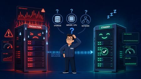
In earlier posts in The Art of Sizing, the focus was on what happens when Oracle systems create their own instability through design shortcuts that seem harmless at first. This post extends that same idea into Data Guard, where a standby database that looks like passive insurance can become part of the foreground performance problem when it is undersized or poorly observed. That is the trap with synchronous disaster recovery. The standby is not just sitting there waiting for a failover. In MAX AVAILABILITY or MAX PROTECTION with SYNC AFFIRM, the primary commit path is directly dependent on the standby receiving redo, writing it to the standby redo log, and acknowledging that write before user sessions are released. When that standby server is short on CPU, struggling on storage, or starved for memory, the latency does not stay isolated on the remote side. It propagates backward into production as log file sync pain, commit stalls, and application slowdown. Why this problem is easy to miss The diagnostic challenge is that the evidence is often sitting on the standby side, but a physical standby in Active Data Guard read-only mode does not behave like a normal local AWR source. Standard local AWR reporting is not enough, and if Remote Management Framework is not already configured, the team can be in the middle of an incident without the standby visibility they actually need. That is what makes this a sizing topic rather than just a monitoring topic. If the standby participates in the commit path, then its storage behavior, CPU headroom, and buffer pressure are part of the production design whether teams acknowledge that or not. How to expose standby performance in Oracle 19c In Oracle 19c, the practical answer is to enable RMF so the primary can collect standby performance snapshots remotely and store them safely in the primary SYSAUX tablespace. The configuration sequence below is the key setup step that makes standby AWR reporting usable during a real production event. -- 1. Enable Management Pack Access on both instances ALTER SYSTEM SET control_management_pack_access='DIAGNOSTIC+TUNING' SCOPE=BOTH; -- 2. Register Nodes and Establish Topology on Primary EXEC DBMS_UMF.configure_node('NODE_PRIMARY', 'PRIMARY'); EXEC DBMS_UMF.configure_node('NODE_STANDBY', 'STANDBY'); EXEC DBMS_UMF.create_topology('ADG_AWR_TOPOLOGY'); -- 3. Link Remote Topology and Enable AWR Service EXEC DBMS_UMF.register_node( 'ADG_AWR_TOPOLOGY', 'NODE_STANDBY', 'DB_LINK_TO_STANDBY', 'DB_LINK_TO_PRIMARY', 'AS_NODE', 'TRUE' ); EXEC DBMS_WORKLOAD_REPOSITORY.register_remote_database( node_name => 'NODE_STANDBY' ); Once the standby is registered, reports can be generated from the primary by running awrrpti.sql and selecting the standby DBID from the menu. What to watch for in a standby AWR report The most useful way to read a standby AWR during a production slowdown is to correlate primary symptoms with standby evidence. The issue usually presents itself as one of a few recognizable patterns. Primary production symptom Standby AWR red flag Likely meaning Spike in log file sync and high SYNC transport lag High log file parallel write on the standby, especially above roughly 5 to 10 ms The standby storage tier is underperforming and slowing standby redo log flushes. Primary LGWR stalls on LNS wait on send Standby host CPU utilization near 100 percent or a high load average The standby is CPU-starved and RFS processes are not acknowledging packets quickly enough. Commit stalls appear at particular hours High ASH on the standby from user reporting activity Heavy Active Data Guard reporting is taking CPU and buffer cache away from recovery work. Flush delays and transport buffer saturation High free buffer waits or checkpoint completed during MRP Buffer cache is too small or DBWR is saturated on the standby. The sizing lesson underneath the incident The bigger lesson is that standby design is not a secondary hardware conversation. In synchronous architectures, the primary database is only as fast as the weakest link in the standby path. That means a disaster recovery platform should not be treated as a low-priority landing zone built from slower storage, thinner CPU allocation, or loosely governed reporting workloads. If it participates in commit acknowledgment, it participates in production performance. The practical operating principles are straightforward: Keep the standby infrastructure performance-symmetric with production where synchronous protection is required. If Active Data Guard is used for reporting, govern those read workloads so they cannot starve RFS or MRP activity. Enable RMF-based standby AWR collection before there is a crisis, not during one. Final thought A standby database is supposed to be your safety net. But in synchronous Data Guard, a poorly sized or poorly monitored standby can become part of the outage story itself. That is the real point here: availability architecture is still performance architecture, and the standby is still part of the sizing equation. That is also why this topic belongs in The Art of Sizing series. Good sizing is not just about capacity. It is about understanding which components quietly sit inside the critical path, and making sure they are designed, monitored, and governed accordingly. Sources The Art of Sizing Data Guard and the Hidden Cost of Small Redo Decisions112Views0likes0CommentsClaude Code as Database SRE: Catching What Your Monitoring Never Will with Everpure Fusion MCP
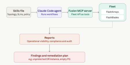
Your DR site might be quietly unprotected and no alert will tell you. That's the gap Anthony Nocentino, Principal Architect at Everpure, Microsoft Data Platform MVP, and self-described computer nerd set out to catch. He built a Database SRE agent using Claude Code and the Everpure Fusion MCP server to audit SQL Server fleets against compliance policy, uncovering a silently unprotected DR instance before disaster struck. Read the full report at "Using Claude Code as a Database SRE Agent with the Everpure Fusion MCP Server"36Views0likes0CommentsEnterprise Storage for Kubernetes: Extending FlashArray Excellence with Portworx Enterprise
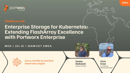
Register Now - July 15! Your FlashArray is already delivering the performance, reliability, and data services your organization depends on. Now Kubernetes is coming to your environment and your applications are following. The question isn’t whether to support stateful Kubernetes workloads. It’s how to do it without sacrificing the storage control, visibility, and SLAs you’ve spent years building. In this live Hands-on Lab, we’ll show storage administrators how Portworx Enterprise (PXE) extends your FlashArray investment directly into Kubernetes. You’ll walk away knowing how to: Provision and manage persistent storage for stateful Kubernetes workloads backed by FlashArray performance Leverage Cloud Drives and StorageV2 to build flexible, scalable storage pools that fit your existing architecture Enforce storage policies and QoS across application teams with Application IO Control and multi-tenancy guardrails Automate capacity management with Portworx Autopilot — so volumes grow on demand without manual intervention or after-hours firefighting Whether you’re being asked to support your first Kubernetes namespace or managing a fleet of clusters, this session gives you a practical, storage-admin-first view of how to extend your FlashArray expertise into the Kubernetes era. Register Now - July 15!77Views0likes0CommentsEnterprise Storage for Kubernetes: Extending FlashArray Excellence with Portworx Enterprise
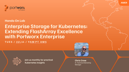
Register Now - July 14th! Your FlashArray is already delivering the performance, reliability, and data services your organization depends on. Now Kubernetes is coming to your environment and your applications are following. The question isn’t whether to support stateful Kubernetes workloads. It’s how to do it without sacrificing the storage control, visibility, and SLAs you’ve spent years building. In this live Hands-on Lab, we’ll show storage administrators how Portworx Enterprise (PXE) extends your FlashArray investment directly into Kubernetes. You’ll walk away knowing how to: Provision and manage persistent storage for stateful Kubernetes workloads backed by FlashArray performance Leverage Cloud Drives and StorageV2 to build flexible, scalable storage pools that fit your existing architecture Enforce storage policies and QoS across application teams with Application IO Control and multi-tenancy guardrails Automate capacity management with Portworx Autopilot — so volumes grow on demand without manual intervention or after-hours firefighting Whether you’re being asked to support your first Kubernetes namespace or managing a fleet of clusters, this session gives you a practical, storage-admin-first view of how to extend your FlashArray expertise into the Kubernetes era. Register Now!67Views0likes0CommentsThe Art of Sizing: Data Guard, Redo Storms, and the Hidden Cost of Bursty Commits
In the previous edition of The Art of Sizing, I focused on redo log switches and why they are so often blamed on storage first. This post extends that same discussion into Oracle Data Guard, where small sizing decisions on the primary database can grow into larger architectural issues across both sites. What begins as an undersized redo design can quickly show up as commit latency, transport sensitivity, standby stress, and misleading storage symptoms. That is the central lesson of Data Guard sizing: the standby does not just replicate business activity. It also replicates the quality of the redo design underneath it. When the redo layer is stable and appropriately sized, Data Guard behaves predictably. When redo is bursty, logs are too small, and switches occur too often, Data Guard magnifies the weakness rather than hiding it. Why Data Guard exists Oracle began shipping standby database capability in the Oracle 8.0.4 era, and by Oracle9i it had evolved into Oracle Data Guard as a formal disaster recovery and availability framework with stronger automation and management capabilities. Its purpose was clear: organizations needed a supported way to maintain a remote copy of production data for failover, switchover, and business continuity without relying on improvised processes around archived redo streams alone. That purpose remains the same today. Data Guard is designed to preserve recoverability and availability, but it does not remove the physical realities of latency. Network round-trip time still matters. Remote acknowledgment still matters. Standby write latency still matters. If the primary database is generating redo in sharp, repetitive bursts while cycling through undersized logs, Data Guard will expose that weakness very quickly. The three transport modes and where commit actually waits Before looking at storms and bursts, it helps to ground the discussion in the three common transport models. Figure 1 shows the practical difference between SYNC AFFIRM, SYNC NOAFFIRM, and ASYNC: not just how redo is transported, but where the acknowledgment point sits relative to the foreground commit path. Figure 1: Oracle Data Guard transport modes showing the acknowledgment point for SYNC AFFIRM, SYNC NOAFFIRM, and ASYNC. In SYNC AFFIRM, the primary commit waits until the standby has performed a durable remote write before the user receives a successful commit response. That provides the strongest protection model of the three, but it also creates the highest commit latency because the foreground path now includes local redo handling, network transport, standby receive processing, standby redo log writes, and remote disk acknowledgment. In SYNC NOAFFIRM, the transport remains synchronous, but the commit can clear once the standby has received the redo into memory rather than waiting for a remote disk flush to complete. That reduces latency compared with AFFIRM while preserving synchronous transport behavior. In ASYNC, the primary does not wait for remote acknowledgment in the foreground commit path. That produces the lowest commit latency, but it also introduces a possible data-loss window if the primary fails before the redo is fully transported and protected at the standby site. The practical takeaway is straightforward. If the business requirement is near-zero or zero data loss and the network and standby design can support it, AFFIRM may be appropriate. If synchronous behavior is required but remote disk flush latency is too expensive, NOAFFIRM is often the more balanced operational choice. If foreground response time matters more than immediate remote durability, ASYNC is usually the cleanest fit. Why redo sizing matters so much This is where many environments make a costly mistake. Teams often treat transport mode as the primary design decision while treating redo log sizing as background plumbing. In reality, redo log sizing is one of the strongest predictors of whether Data Guard feels stable or painful under load. Long-standing Oracle practice is clear: a healthy system should not be switching redo logs constantly. A normal target is roughly 3 to 5 switches per hour during peak activity, not a switch every minute or two. Once switch frequency becomes excessive, Oracle begins manufacturing its own turbulence. Every switch drives checkpoint advancement, dirty buffer flushing, control file updates, and archiver coordination. That churn is disruptive even on a standalone system. In a Data Guard architecture, it becomes a cross-site problem. Earlier telemetry showed that sustained redo rates in the range of about 34 MB/s to 39 MB/s, combined with undersized logs, were enough to create a switch-storm pattern and the kind of latency that often gets blamed on storage first. What a Data Guard switch storm looks like Figure 2 makes that switch storm visible. It shows a database switching roughly 40 times per hour compared with a best-practice target of around 3 to 5 switches per hour. More importantly, it shows that both SYNC AFFIRM and SYNC NOAFFIRM suffer from the same local Oracle storm on the primary side: repeated checkpoint work, ARCn pressure, control file activity, and rising commit latency. The real difference is not whether the local storm exists, but where the remote acknowledgment point sits in the commit path. Figure 2: Data Guard under a redo log switch storm, showing how 40 switches per hour drive repeated checkpoint pressure, ARCn pressure, and commit latency spikes in both synchronous modes. Under SYNC AFFIRM, the pain is greatest because the foreground commit must survive both the local churn and the full remote durable-write acknowledgment before the user is released. Under SYNC NOAFFIRM, the latency penalty is lower because the remote disk flush is removed from the foreground path, but the primary still absorbs the same switch storm locally. Under ASYNC, the commit may clear quickly, but the standby can still fall behind in transport or apply if redo arrives faster than the downstream system can consume it. Why storage can look healthy while the database feels bad This is the point where DBAs and storage teams often talk past one another. Repeated switch-driven checkpoint waves create short, sharp, bursty I/O patterns rather than a smooth write stream. The array can look healthy on paper. Average latency can look acceptable. The platform may still have plenty of headroom. Yet the database users can still be feeling brief but repetitive stalls every time the redo architecture forces another checkpoint cycle and another wave of coordination work. That is why a fast array does not automatically eliminate the problem. The issue is often not sustained bandwidth exhaustion. The issue is workload shape. If redo arrives in spikes and the logs are too small, the backend experiences bursty pressure rather than a smooth average. Even an excellent array can be difficult to interpret when the real pain occurs in short windows that disappear inside broader averages. This is also why coarse AWR timing can be deceptive. A 15-minute reporting window can smooth dozens of short checkpoint spikes and log-switch bursts into something that looks moderate. If the system is switching every 90 seconds or every couple of minutes, you often need 1-minute granularity, or finer if the tooling allows it, to see the real pattern. Array-side telemetry is especially useful here because it can expose the microburst behavior more clearly than coarse Oracle summaries do. Why SYNC AFFIRM degrades under bursty redo Figure 3 brings the entire problem into focus. It shows why a system with 4 GB redo logs switching more than 40 times per hour can turn what looks like a modest average redo rate into a foreground and background stress event across the Oracle stack and the storage layer. Figure 3: Why SYNC AFFIRM drives high log file sync under bursty redo, showing the burst pattern, the foreground commit chain, switch-generated extra work, and wait propagation across Oracle and the SAN. The first panel shows the source pattern: burst redo rather than a smooth stream. The slide describes 4 GB online redo logs, more than 40 switches per hour, approximately one switch every 1 to 2 minutes, roughly 160 GB of redo per hour, and an average redo rate near 45 MB/s. Its warning is exactly right: the average rate can look modest while the instantaneous pattern is bursty and repetitive. That distinction matters because a database can look reasonable in average throughput terms while performing badly in commit latency. The bursts fill small logs quickly, and each rapid switch triggers another round of local and remote work. The second panel walks the critical SYNC AFFIRM commit path. A foreground user issues a commit. LGWR serializes the commit records. Redo is written to the local primary redo log. It is then transported synchronously to the standby, received by RFS, written to standby redo logs, flushed to disk, and only then acknowledged back to the primary so the commit can be released. In other words, remote durable write is not a side activity in AFFIRM; it is part of the foreground commit path itself. The third panel explains why log file sync gets dramatically worse under this pattern. The wait does not inherit one isolated delay. It inherits the full chain: LGWR serialization, local redo write service time, inter-site RTT and jitter, standby receive service time, standby redo write service time, remote durable flush acknowledgment, and then the repeated switch churn that injects checkpoint, control file, and archiver coordination every 90 seconds or so. The fourth panel makes another important point: this is not just an LGWR issue. Foreground stress appears in user sessions, LGWR, the commit path, log file switch completion exposure, log buffer space pressure, and transaction stall behavior. Background stress lands on DBWn, CKPT, ARCn, RFS, standby redo log writes, and control file sequence metadata work. A switch storm is not a single bottleneck; it is a coordinated pattern of foreground and background pressure. The fifth panel is especially useful for storage teams because it shows the backend write pattern. The SAN is not observing a flat 45 MB/s stream. It is seeing primary redo writes, shipped redo, standby redo writes, archiver rereads after switch, and additional checkpoint-driven datafile writes, with several components shown at roughly 160 GB/hour minimum and checkpoint-driven activity identified as workload dependent and burst amplified. That is why the backend can appear healthy in average terms while still absorbing violent front-end bursts and queue spikes. The sixth panel shows the cascading shape of the workload. A redo burst fills the log. A switch occurs. Extra writes and rereads hit storage and SAN. Foreground commits wait for remote durable acknowledgment in SYNC AFFIRM. Log file sync escalates. The slide describes each switch as producing an echo of extra work, and that is an accurate way to think about it. The stress symptoms listed on the right side of the slide align closely with what experienced teams often see during these events: very high log file sync, elevated log file switch completion waits, log buffer space pressure, sensitivity in SYNC remote write or redo transport, SAN queue bursts, and front-end write spikes. The key lesson is that local write latency alone may not look catastrophic, yet the foreground commit experience can still become severe because the full path is waiting on the entire chain to clear. What improves when redo logs get larger The encouraging part of the story is that the operating pattern can be improved significantly even when the protection model stays the same. Figure 4 shows the outcome teams actually want: the same workload, the same SYNC AFFIRM design, but far fewer self-inflicted switch events because the online redo logs are larger. Figure 4: Modeled impact of increasing online redo logs under SYNC AFFIRM, showing that redo volume remains similar while switch frequency, checkpoint turbulence, and burst-driven array stress fall materially. The comparison is straightforward. At roughly the same redo generation volume of about 160 GB per hour, moving from 8 GB logs to 40 GB logs reduces the switch rate from about 20 switches per hour to about 4 switches per hour. That changes the approximate switch interval from around 3 minutes to around 15 minutes while keeping the commit path mode the same: SYNC AFFIRM. The protection model has not changed, but the operating pattern has. Checkpoint wave frequency becomes much lower. Archiver wakeups and control-file churn become much lower. The array-facing write pattern becomes flatter and less bursty. The workload-shape panel is especially valuable because it shows that redo volume is not the same thing as switch turbulence. With 8 GB logs, the environment hits repeated switch boundaries and repeated checkpoint flush waves throughout the hour. With 40 GB logs, those boundaries are much less frequent, the checkpoint waves are much less repetitive, and the system spends far less time manufacturing its own instability. That reinforces the core message of this post: many Data Guard performance problems are not caused by total redo volume alone. They are caused by the shape of the workload and by how often Oracle is forced to react to full logs, checkpoints, archiver cycles, and control-file updates. The Oracle task impact model in the slide also matches real-world behavior. With larger logs, LGWR commit pressure is lower, log file sync exposure is lower, CKPT activity is much lower, DBWn flush pressure is much lower, ARCn archive pressure is much lower, control-file update churn is much lower, and log switch completion risk is much lower. This does not mean larger logs magically remove the cost of SYNC AFFIRM. The caveat panel in the slide is correct: if remote AFFIRM acknowledgment remains the dominant bottleneck, log file sync may improve only partially. But checkpoint, archiver, and control-file churn should still drop materially, and the write pattern presented to the array should smooth out. That is the practical point storage teams need to see. A larger redo configuration does not reduce the need for remote durable acknowledgment in SYNC AFFIRM, but it does reduce the self-inflicted switch overhead around that acknowledgment path. In many environments, that is enough to materially reduce front-end write burstiness, queue depth volatility, in-flight spike risk, and visible host-side latency spikes. Final thought Data Guard is a very capable product, but it is also brutally honest. It reflects the quality of the primary redo design with very little mercy. If the logs are too small, the switches are too frequent, and the workload is bursty, SYNC AFFIRM will make that weakness highly visible by placing remote durable acknowledgment inside an already stressed commit path. The array may be fast. The network may be fast. The standby may be healthy. But if the redo architecture is wrong, the full chain can still stall. That is the real art of sizing Data Guard. It is not just about how much redo is generated. It is about how that redo arrives, how quickly logs fill, how often switches occur, where the acknowledgment point sits, and whether the measurement tools are granular enough to reveal the truth before averages hide it. Sources Oracle Log Switch Architecture Analysis & Blog Framework Storage Performance & Redo Architecture Root Cause Analysis V2 1 Oracle9i Data Guard Concepts Oracle 9i - Oracle FAQ racle 11g Data Guard and RAC Oracle Redo Log Sizing Cost-Benefit & Performance Savings Analysis161Views0likes0Comments